Question 1

How to Add New Rows ?

ammaranass · Accepted Answer

METHOD 1: USING THE RIBBON MENU

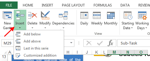
From the ribbon menu, click on « Add Tasks » then pick the desired option:

Add below: a new task will be added below the selected row
Add above: a new task will be added above the selected row
After the last row: a new task will be added after the last row of the task group
Customized menu: an advanced menu will be displayed with much more options

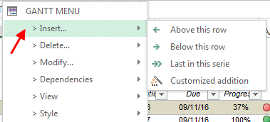
This menu is also available from the right click drop down list:

METHOD 2: COPY – PASTE EXISTING ROWS

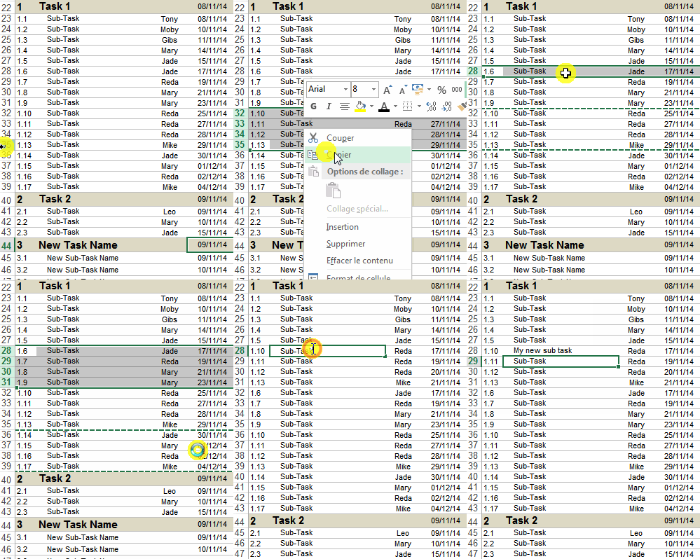
Select any row from the Gantt Chart (you can select more than 1 row if necessary), right click ans then click on Copy. Once done, select destination row, right click and select « Insert Copied Cells ».

Did you find a solution to your question ? Link to the contact form Back to the top of the page

Question 2

How to Change the Starting date of the Gantt Chart ?

ammaranass · Accepted Answer

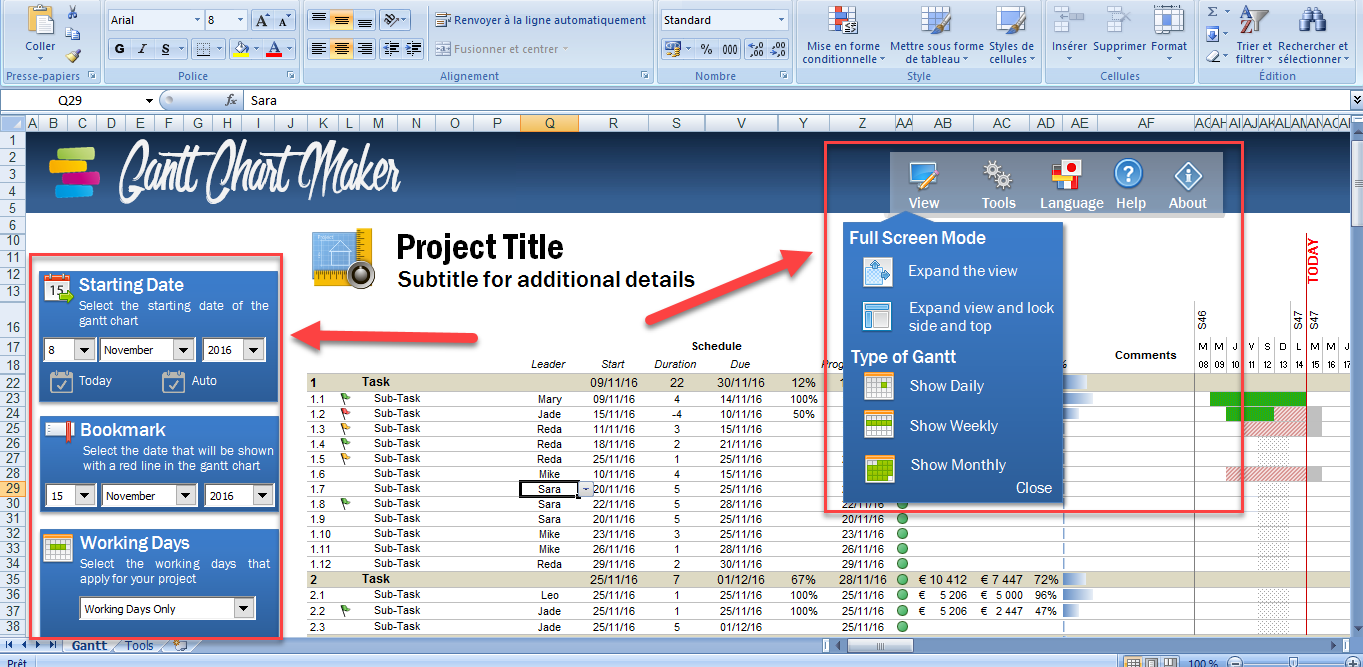
To change the start date of the gant chart, use the ribbon menu:

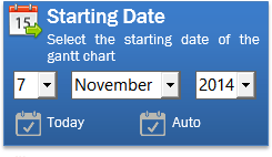
Or the left menu:

You may consider to just click on « Auto »: the macro will automatically look for the earliest date in your planning and set it as a starting date. From time to time, you can click on this icon to reflect the latest updates you make to your chart. Another way is to click on « Today ». The Gantt Chart will use today date as a starting date. Did you find a solution to your question ? Link to the contact form Back to the top of the page

Question 3

How to Input the Start Date of a Task ?

ammaranass · Accepted Answer

MANUAL INPUT

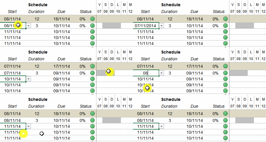
You can manually input any date as a starting date of task. Select the appropiate cell and type the starting date. If there is already another date or another formula inside this cell, you can safely overwrite it. Once you update the starting date, the gantt chart will reflect automatically this new input.

USING THE MENUS:

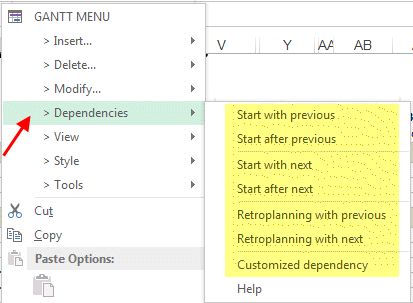
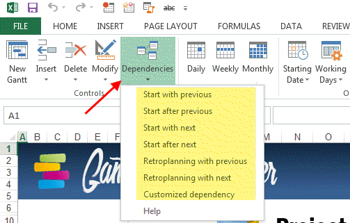
You can also decide to use the drop down list from the ribbon menu. Select the subject task then click on « Dependencies » and choose the appropriate option.

You can access this menu from the right-click drop down list as well:

From this list, you can pick your desired option:

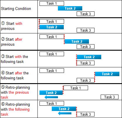
After the previous task: the task will start after the previous one
With the previous task: the task will start at the same date as the previous one
After the following task: the task will start after the following one
With the following task: the task will start at the same date as the following one
Retroplanning with the previous task: the subject task will end with the start of the previous task
Retroplanning with the following task: the subject task will end with the start of the following task
Customized dependency : will open a specific menu that can link tasks between them

For more details about dependencies, refer to "How to set dependencies (or constraints) between tasks ?".

USING FORMULAS:

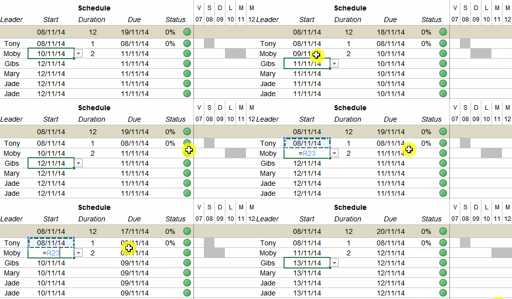
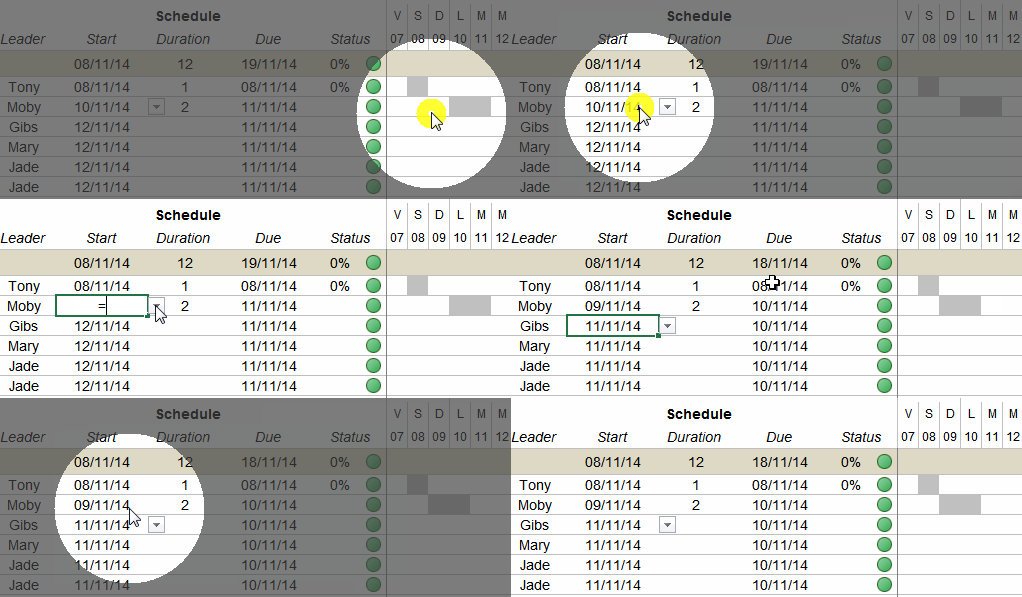
For more flexibility, you can opt to set-up simple formulas to link different tasks or sub-tasks:

Select the cell that contains the « Start Date » that you would like to modify
Write the symbol equal « = »
Select any other date (« Start Date » or « End Date »)
Write +1 (to add one day)
Confirm by pushing « Entry » key

For example, if you would like to start a sub-task after the previous one, these are the steps to follow:

Based on the above example; you can play with this formula by adding or substracting more or less than 1 day. Also, instead of linking to the previous sub-task, you can make a link with any other cell of your table.

Did you find a solution to your question ? Link to the contact form Back to the top of the page

Question 4

How to Input a Duration ?

ammaranass · Accepted Answer

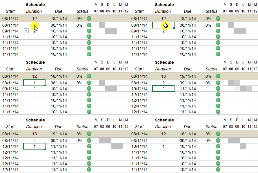
Inputting a duration is quite straight forward: just select the appropriate cell and input the desired number of days. The gantt chart will be updated automatically. The Gantt Chart will also consider which working days you selected: Monday to Friday or Monday to Sunday.

The end date is automatically calculated via a formula which uses:

The Starting date
The Duration
The type of calculation (Working Days, which days are weekend days)

In case you would like to build the schedule in retro-planning (starting from the end and building the schedule backward) you can opt for negative duration:

Input the last day of the task in the cell « Start Date »
Input the desired duration with minus symbol : for example -5

Did you find a solution to your question ? Link to the contact form Back to the top of the page

Question 5

How to Update the Progress Status of a Task ?

ammaranass · Accepted Answer

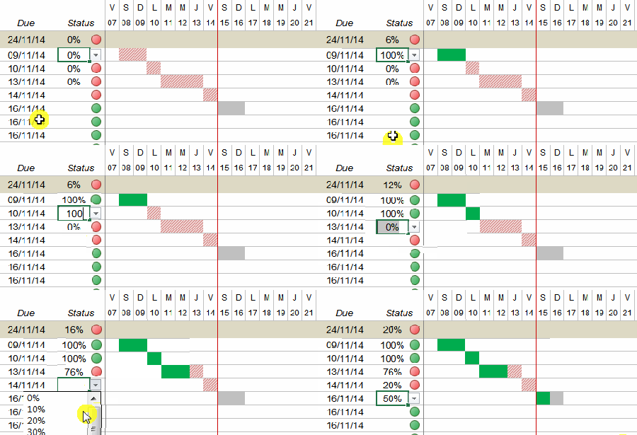
From the drop down list, select the progress status of any sub-task. You can also manually input any value you would like by selecting the cell and entering the desired percentage. This information will be used to check if a task is on-track or in delay:

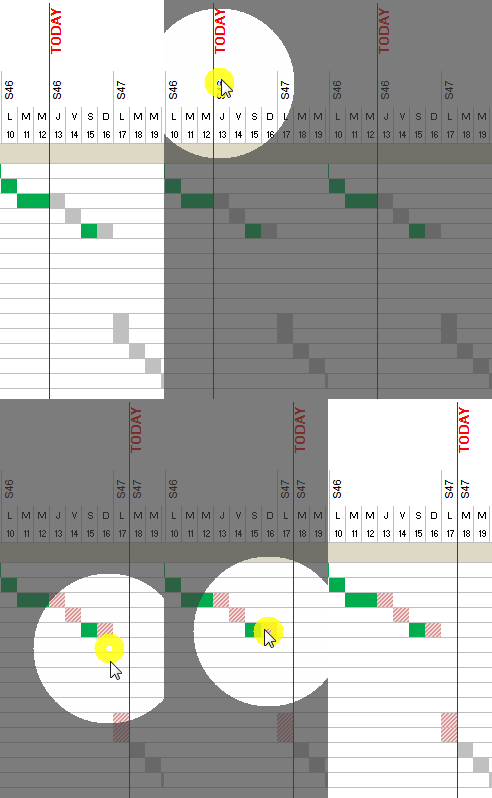
If the task is behind the red line (a line which reflects your specified today’s date), then the completed portion will be shown in green and the rest in hashed red ;
If the task is not behind schedule, it will be shown in green and grey

The round shapes next the percentage follow the same logic. If you wish to not distinguish tasks in delay, just set the « Baseline » to a date in the far future (e.g: 01/01/2020). If so, all tasks will show in green and grey. Did you find a solution to your question ? Link to the contact form Back to the top of the page

Question 6

How to Assign a Responsible Person ?

ammaranass · Accepted Answer

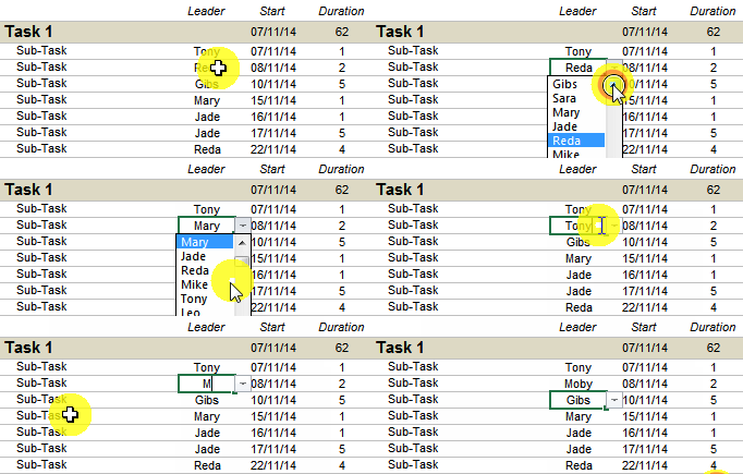
For any task, you can choose from a drop down list the name of the responsible person. If the name of the responsible person is not in this list, you can over-write manually any name you would like to.

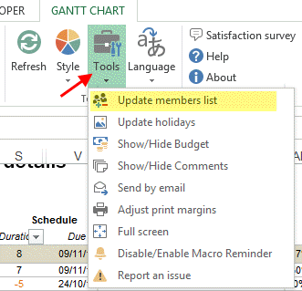
The drop-down list is based on the informations about project members. This list can be accessed by a click on « Tools » and « Update Members List ».

Did you find a solution to your question ? Link to the contact form Back to the top of the page

Question 7

How to re-number the tasks ?

ammaranass · Accepted Answer

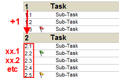
When you add a new set of tasks, the Gantt Chart Maker use the previous task number and increment it:

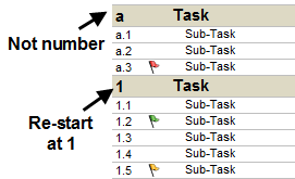
If the previous task number is not numerical, then the new series is numbered with 1:

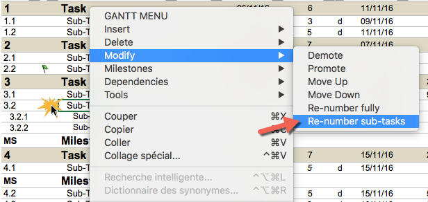
To update the numbering (e.g: after a while the tasks are not numbered correctly, you would like to use your own numbering system), you can follow the below step:

Start with allocating a task number or reference for each task (the head of each task set)
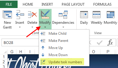
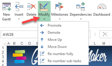
Use the function « Modify -> Update the numbering » from the right click menu or from the ribbon menu

From the ribbon menu:

Did you find a solution to your question ? Link to the contact form Back to the top of the page

Question 8

How to Modify the « Baseline » Date ?

ammaranass · Accepted Answer

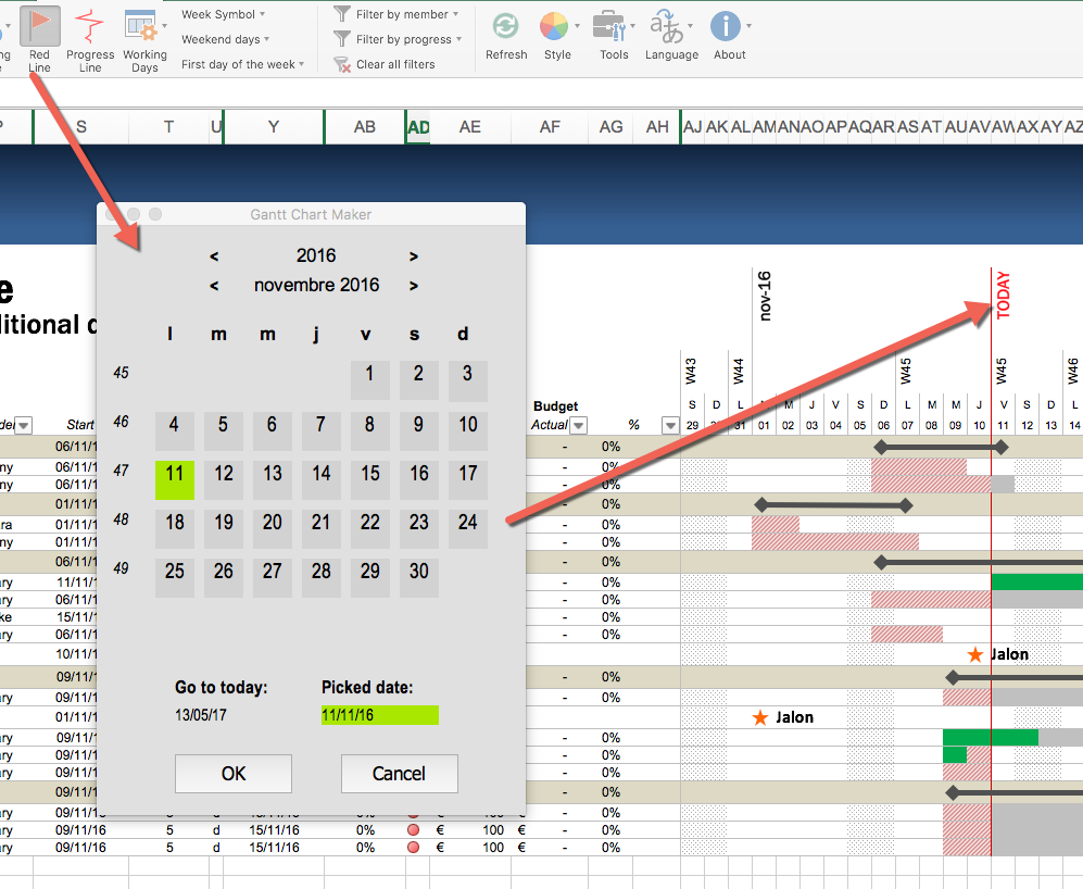
The purpose of the Baseline is to highlight in the gantt chart a specified date that serve as a reference for the complete planning. This date is not necessary the actual today’s date: if your presentation is in 2 weeks, you may consider to already set the baseline to a future date and see how the chart will look like. The baseline is useful to highlight the tasks that are behind schedule and the ones that are progressing according to plan. Basically, any task behind the red line which is not 100% completed is in delay. 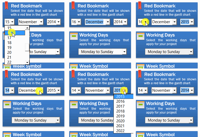If you would like to change this date, select from the left panel an appropriate date:

You can also use the ribbon menu :

Once done, the Gantt Chart will update automatically the red bookmark and also check one more the due dates of all the tasks against this line.

If you would like to completely hide this line from your gantt chart, just set it to a date in the far future (e.g: 01/01/2020). Did you find a solution to your question ? Link to the contact form Back to the top of the page

Question 9

How to Force the Gantt Chart to Refresh the View ?

ammaranass · Accepted Answer

With some computers, it is possible that the Gantt Chart does not refresh properly or frequently enough:

Although you update a starting date, a duration or a status, the Gantt Chart does not reflect these updates
Although you add a flag, the flag does not appear
etc

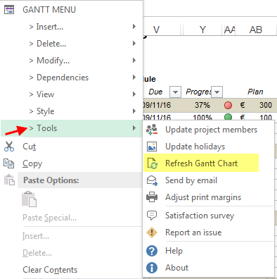
We added a special feature to force Microsoft Excel to refresh all the fields. From the ribbon menu menu, click on the icon «Refresh»:

You can also force this refresh by simply pushing the keyboard keys CTRL + N or using the right click menu:

Did you find a solution to your question ? Link to the contact form Back to the top of the page

Question 10

How to Change the Language ?

ammaranass · Accepted Answer

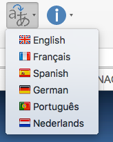
From the ribbon menu, click on « Languages » and then select your language. Currently, six languages are available: English, French, Spanish, German, Dutch and Portuguese.

Did you find a solution to your question ? Link to the contact form Back to the top of the page

Question 11

How to Show and Fill Budget Fields ?

ammaranass · Accepted Answer

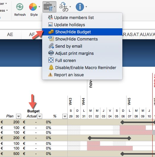
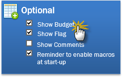
First of all, make sure « Show Budget » option is ticked:

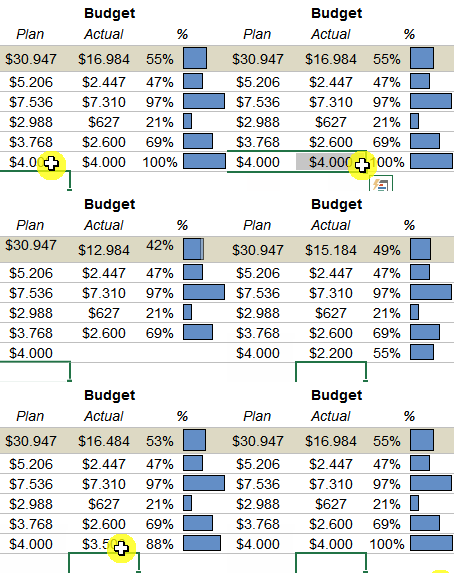
In front of each task or sub-task, you will see budget cells. Simply fill your estimated or planned budget then, whenever you have new information, fill-in the actual consumed budget. Other cells will adjust automatically.

You can change the currency using the usual Excel Formatting. Important notice : When you untick « Show Budget », the macro will only hide the related columns. The content will be kept as it is and any one can still see if he unhides the columns Z, AA and AB. Therefore, if you would like to completely hide such information before sending to an external party, it is recommended that you clear all these information manually (select related cells and push « delete » key). Once it is done, untick « Show Budget ». To remind you about this point, a pop-up message will be shown everytime you untick this feature. This parameter is also available from the left menu:

Did you find a solution to your question ? Link to the contact form Back to the top of the page

Question 12

How to Show/Hide the Column for « Comments » ?

ammaranass · Accepted Answer

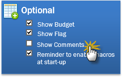
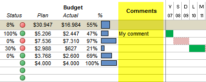
Simply tick or untick « Show Comments »:

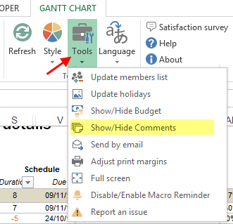
Or from the ribbon menu:

Doing so will unhide/hide the column where you can input free comments for each task:

Did you find a solution to your question ? Link to the contact form Back to the top of the page

Question 13

How to Automatically Share the Latest Schedule by Email ?

ammaranass · Accepted Answer

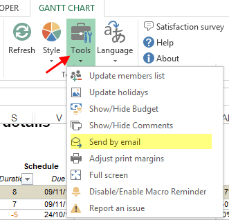
This Excel Gantt Chart Maker has a nice feature that allows you to share your Excel file by email. Click on « Tools » then « Share by email ».

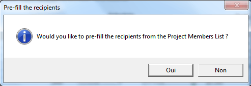
A message will prompt asking you if you would like to pre-fill the recipients field automatically from the members list or not. This is meant to avoid you sending the schedule to all the members while your intention was to send it to few people.

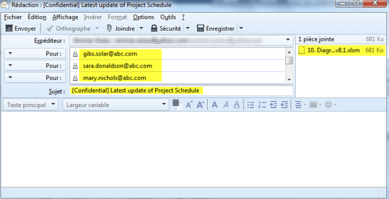
A draft email will be prepared using your default software program. It will not be sent until you complete the remaining fields and click on send.

Did you find a solution to your question ? Link to the contact form Back to the top of the page

Question 14

How to add a new gantt chart in the same file ?

ammaranass · Accepted Answer

It is possible to have multiple Gantt Charts in the same file. To add a new Gantt Chart, click on icon « New Gantt Chart » from the ribbon menu.

It is also possible to use the usual copy-paste function of an existing sheet. Did you find a solution to your question ? Link to the contact form Back to the top of the page

Question 15

How to Reach the support page from the Gantt Chart Maker ?

ammaranass · Accepted Answer

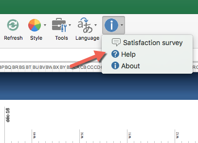
From the ribbon menu, click on the icon « About » and then « Help ». You will be transferred to the support page which contains a FAQ that is regularly updated.

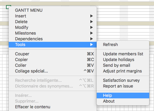
You may also use the right click menu:

Did you find a solution to your question ? Link to the contact form Back to the top of the page

Question 16

Is it possible to input task durations in weeks or months ?

ammaranass · Accepted Answer

It is possible to input task durations in days, weeks or months. Ideally it is better to input these durations in days but if your planning does not allow such precision level you can input them in weeks or in months. Next to any duration there is a letter "d" which means "days". If you double click on it you will change it to "w" (weeks) or "m" (months).

Did you find a solution to your question ? Link to the contact form Back to the top of the page

Question 17

What is the purpose of a "Milestone"

ammaranass · Accepted Answer

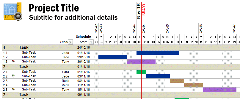
Milestones are tools used in project management to mark specific points along a project timeline. These points may signal anchors such as a project start and end date, a need for external review or input and budget checks, among others. In many instances, milestones do not impact project duration. Instead, they focus on major progress points that must be reached to achieve success. A "Milestone" is visualized in the Gantt Chart Maker with a star mark (milestone does not have a duration):

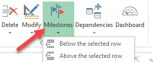
To add a new milestone, click on the icon "Milestone" from the ribbon menu:

In case you would like to change an existing task to a Milestone, click on the icon "Modify" then "Promote" until the task become a milestone.

Did you find a solution to your question ? Link to the contact form Back to the top of the page

Question 18

How to copy/paste tasks between different gantt charts ?

ammaranass · Accepted Answer

When you copy/paste tasks from different gantt charts, you will get a warning message similar to the one below:

Just click on the button "Yes": it will not have any impact on your file. Did you find a solution to your question ? Link to the contact form Back to the top of the page

Question 19

I can't see the ribbon menu (Excel 2007 & Mac 2008)

ammaranass · Accepted Answer

Due to technical reasons, the ribbon menu is not available on Excel 2007 (PC) and 2008 (MAC). Ideally, if you could upgrade to at least Excel 2010, you will benefit from a much better user experience. However if you can't migrate from Excel 2007 or 2008 (e.g: company policy) you may still use the Gantt Chart Maker through the right and the left menus that are available on the sheet itself :

Malgré que le menu ruban n'existe pas sur Excel 2007, il est possible de contrôler l'outil depuis les différents menus existant :

Did you find a solution to your question ? Link to the contact form Back to the top of the page

Question 20

How to Show the Chart Weekly, Daily, Monthly, Quarterly ?

ammaranass · Accepted Answer

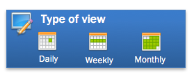
From the ribbon menu, choose « Weekly », « Daily », « Monthly » or « Quarterly »:

This parameter is also available from the left side menu:

Did you find a solution to your question ? Link to the contact form Back to the top of the page

Question 21

How to Change Project Title and Logo ?

ammaranass · Accepted Answer

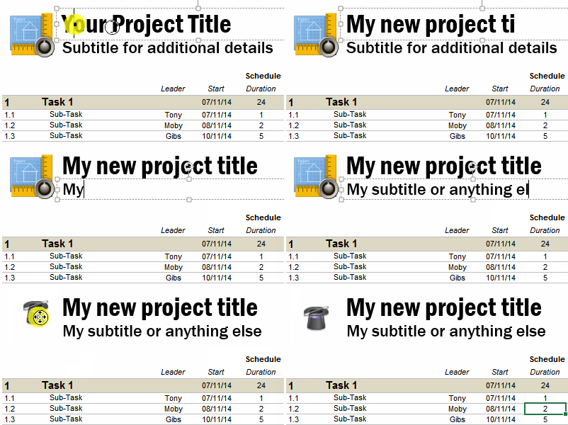
To update your project title, just change directly the content of the textbox. For the logo, delete the current one and insert a new picture using the usual Excel functions.

Did you find a solution to your question ? Link to the contact form Back to the top of the page

Question 22

How to Add a Flag to a Tasks ?

ammaranass · Accepted Answer

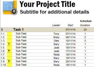
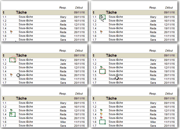
As a project manager, for prioritization, you will not only base yourself on fact and figures but eventually on your intuition as well. These red, orange and green flags are not linked to any rule or formula: you can freely choose any of these flags.

In front of any task, use a double click on the cell until you pick the desired flag (green > yellow > red > nothing). A second method consists in inputting in the flag cell a value from empty or 1 to 3:

1: green
2: yellow
3: red
empty: nothing

If you would like to add a flag to many cells, you can use copy-paste. To deleted several flags, select them and push the delete key.

Did you find a solution to your question ? Link to the contact form Back to the top of the page

Question 23

How to Modifiy the Way Weeks Numbers are Displayed ?

ammaranass · Accepted Answer

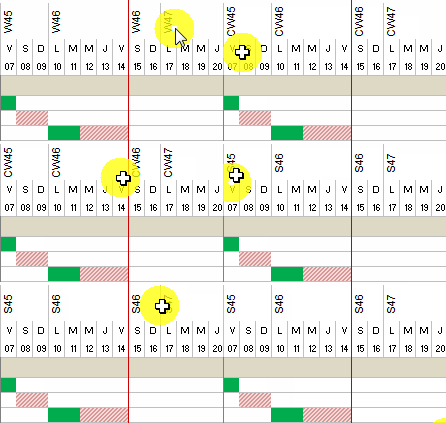
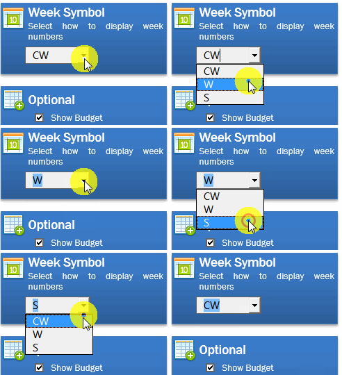
Weeks numbers can be displayed in several ways:

W45 : Week 45
CW45 : Calendar Week 45
S45 : For French and Spanish

To select the appropriate one, choose from the ribbon menu one of the three available options:

This parameter can be also set-up from the left menu:

Did you find a solution to your question ? Link to the contact form Back to the top of the page

Question 24

How to Automatically Adjust Print Margins ?

ammaranass · Accepted Answer

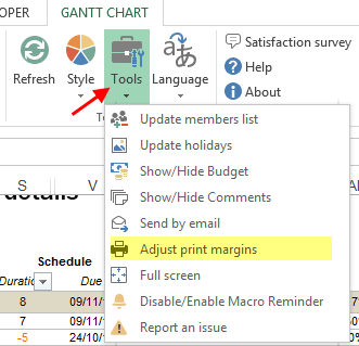
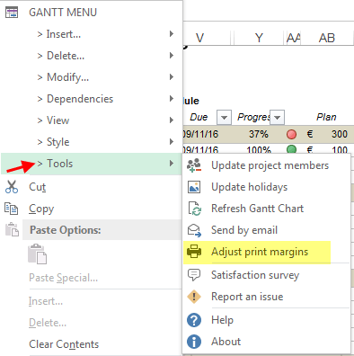
It can be frustrating to adjust the print margins evrytime the schedule shorten or widen. Therefore we have included a macro that (literally) reads all the dates of the gantt charts and find out for you which last row and which last column should be considered for the print out. Simply click on « Tools » and « Adjust Print Margins »:

And from the right click drop down list:

Did you find a solution to your question ? Link to the contact form Back to the top of the page

Question 25

How to Modify Working Days (week days) ?

ammaranass · Accepted Answer

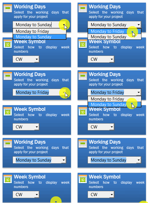
To choose the working days that apply to your project, click on the icon « Working Days » then choose « Monday to Friday » or « Monday to Sunday ».

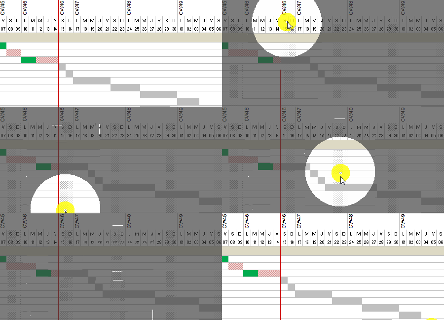
The Gantt Chart will adjust automatically. If Saturday and Sunday are non-working days, they will be greyed-out.

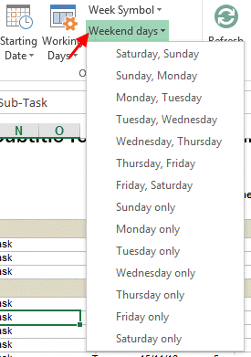
By default, week-end days are "Saturday and Sunday". If you would like to modify this choice, choose from the ribbon menu a different parameter:

Did you find a solution to your question ? Link to the contact form Back to the top of the page

Question 26

How to Modify Holidays and Vacations ?

ammaranass · Accepted Answer

This Gantt Chart Maker is able to exclude holidays when calculating a duration. These holidays can be:

Bank holidays
Shut down periods of the company
Any other vacation period you want to exclude

First of all, as a pre-requisite, the gantt chart should be set-up as « Working Days Only » (Monday to Friday). This parameter can be set from the ribbon menu:

Or the left side menu:

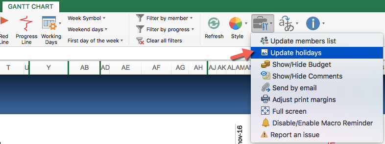
Then, to set-up these holidays dates, click on the icon « Update Holidays »:

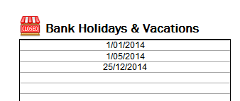
You will be transferred to the « Tools » sheet where you can update the holidays that apply to your project. You can enter any date you would like to consider as holiday, vacation or shut-down period. These dates need to be entered individually:

If the project members will be on vacation from 24th of December till 2nd of January, you should input each day gf this period in an individual row

In the Gantt Chart, these days will be greyed-out in the same way as Saturdays and Sundays. Did you find a solution to your question ? Link to the contact form Back to the top of the page

Question 27

How to extend the Gantt Chart period ?

ammaranass · Accepted Answer

By default, the gantt chart has 557 columns which represent roughly 18 months. Even your project is more than 18 months, it is possible to visualise it by changing the "Starting Date" of the chart and slide the visible portion. Another way is to extend the period of the Gantt Chart by adding new columns on the right side of the chart:

Select the last column of the chart
Copy
Select as many empty columns as you would like
Paste
Refresh

[video width="1530" height="696" mp4="https://www.mgt-tools.com/wp-content/uploads/2017/05/agrandir-droite-EN.mp4"][/video] Did you find a solution to your question ? Link to the contact form Back to the top of the page

Question 28

How to hide the left menu ?

ammaranass · Accepted Answer

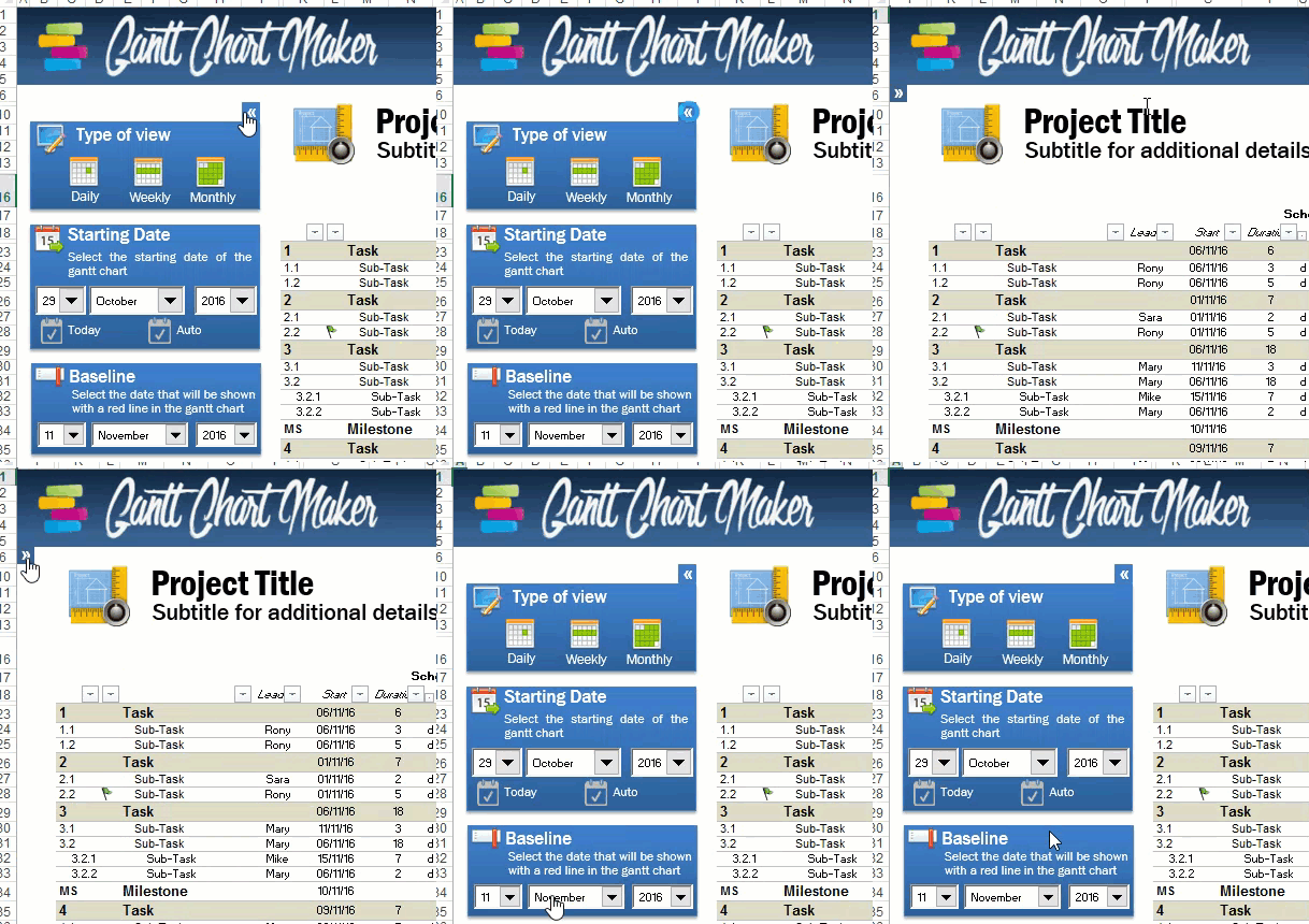
To hide/show the left menu click on the icon "«":

Did you find a solution to your question ? Link to the contact form Back to the top of the page

Question 29

How to migrate to a new version of the tool ?

ammaranass · Accepted Answer

The Gantt Chart Maker is regularly updated in order to add new features or fix minor bugs. When a new version is released, it is generally possible to migrate from the old to the new version.

Make sure you saved a back=up copy of your files
Open both files: new and old version
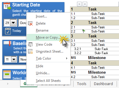
From the old version, right click on the sheet you would like to copy then click on "Move or Copy"
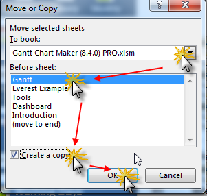
From the next window choose the filename containing the new version, "Create a copy" then "OK"

Note: We put lot of efforts to make it possible to migrate from old to new versions however this migration is not always possible in the case of significant improvements to the sheets. We will highlight this situation by a major version change (e.g: version 7.5 to 8.0). If the migration is not possible with copy/paste of the sheets, it is still possible to do it manually by copy/paste each row containing your data.

Did you find a solution to your question ? Link to the contact form Back to the top of the page

Question 30

How to repair formulas ?

ammaranass · Accepted Answer

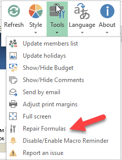
After some time, it can happen that the excel formulas used in to calculate the Gantt Chart are not correct anymore. Formulas includes the ones that calculate budget totals/sub-totals, duration of tasks, etc If you would like to repair those formulas that are usually automatically calculated by the tool you may consider using the feature called "repair formulas" :

Before using this feature, please back-up your document as any manual input in the cells that are supposed to hold formulas will be overwritten. Did you find a solution to your question ? Link to the contact form Back to the top of the page

Question 31

How to Activate/Deactivate the Reminder about « Enable Macros »?

ammaranass · Accepted Answer

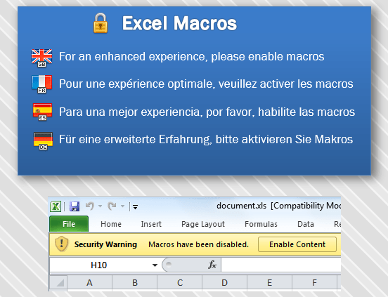
Everytime the Gantt Chart Maker is opened, a reminder is displayed to ask the user to enable macros.

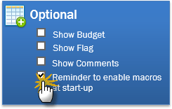
Purpose of this reminder is to avoid the usage of the Gantt Chart Maker without the macros enabled which may impact the quality of the tool or give the impression that the file is not working properly. This is quite useful when someone is using this tool for the first time or in case you send this file to a project stakeholder not familiar with such document. The only drawback to this reminder is that it saves the file everytime you close it, whatever the condition is. If this limitation is not suitable for your requirements, you may want deactivate this reminder. To do so, simply untick the box in the « Optional » menu:

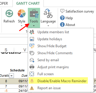
This parameter is also available from the ribbon menu:

Did you find a solution to your question ? Link to the contact form Back to the top of the page

Question 32

How to Customize the Colors Used in the Gantt Chart?

ammaranass · Accepted Answer

FROM THE MENUS:

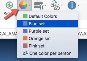
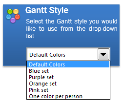
From the ribbon menu « Style », pick one of the 6 pre-set colors:

Default: Green, Grey and Red
Blue
Purple
Orange
Pink
One color per person in charge: each team member can have his own color in the Gantt Chart

This option is also available on the left menu:

ADVANCED METHOD:

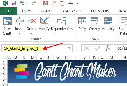
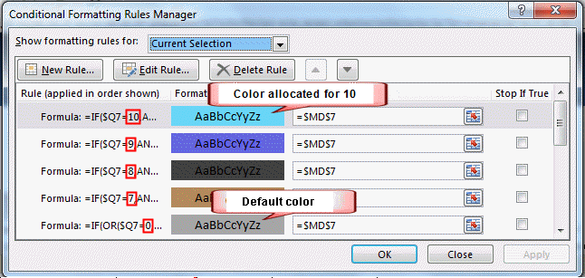
If you would like to further customize these colors, follow the below steps. In the area « Name Box » (top left area of Excel), input exactly the following name: « CF_Gantt_Engine_1 » then push Enter.

The value « CF_Gantt_Engine_1 » corresponds to the default colors (Green, Grey and Red). If you would like to modify other pre-set colors, you need to select one of the below option:

CF_Gantt_Engine_2 : blue colors
CF_Gantt_Engine_3 : purple colors
CF_Gantt_Engine_4 : orange colors
CF_Gantt_Engine_5 : pink colors
CF_Gantt_Engine_6 : « One color per person in charge »

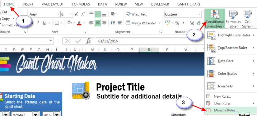
Then from the Excel Ribbon menu, click on « Conditional Formatting » then « Manage Rules »:

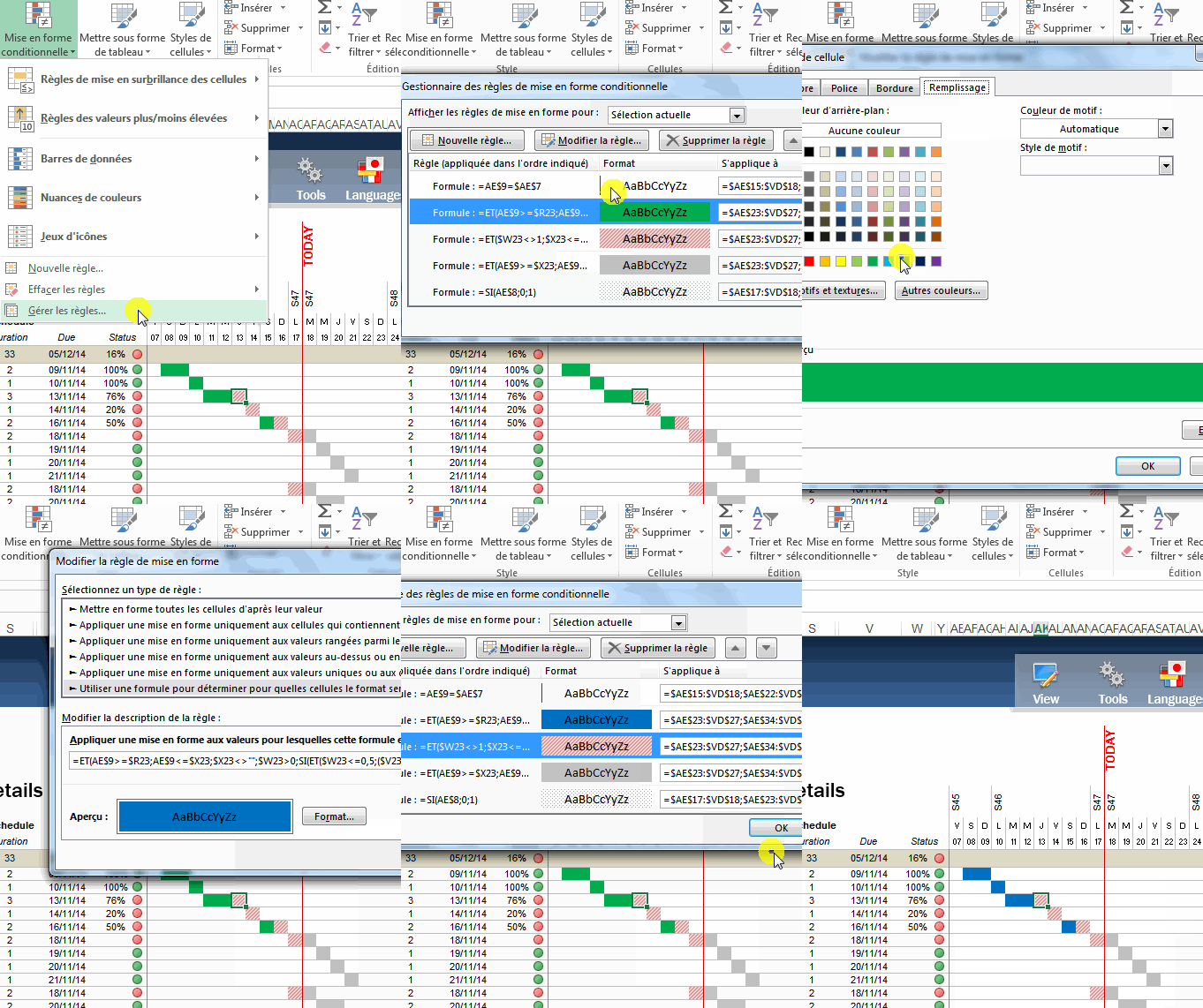
Scroll down until you see a color you would like to modify. Then click on « Edit the rule ». As of then you can change anything you wish related to this rule.

To update the Gantt Chart, click on refresh from one of the available buttons:

Did you find a solution to your question ? Link to the contact form Back to the top of the page

Question 33

How to customize the pre-defined colors of « one color per person in charge » ?

ammaranass · Accepted Answer

THE EASIEST WAY:

The pre-defined set-up « one color per person in charge » allocate to each person one specific color. This visualization helps in identify who is responsibly for what.

In order to not overload the calculations, this method can take up to 10 different persons in charge. The color allocated for each person in visible in the sheet named « Tools »:

You can modify the color of each person by allocating a number from 1 to 10. You can allocate the same color to more than one person if needed (e.g: all QA members can have the same color). If the cell is left blank or if you allocate a number which is not in the range 1-10 then the default color will be used (grey).

ADVANCED METHOD:

Beyond the method described above, you can customize the actual colors. To do so, you would need to follow the step-by-step explanation given to the FAQ : "HOW TO MODIFY THE COLORS OF THE GANTT CHART MAKER" . Use the parameter « CF_Gantt_Engine_6 ». This advanced method will allow you to modify the color that are allocated to each figure from 1 to 10:

Did you find a solution to your question ? Link to the contact form Back to the top of the page

Question 34

How to set dependencies (or constraints) between tasks ?

ammaranass · Accepted Answer

A dependency is a logical relationship between 2 tasks or between a task and a milestone. In the Gantt Chart Maker, 6 types of dependencies exist:

METHOD 1: SET A DEPENDENCY BETWEEN TWO ADJACENT TASKS

The easiest way to set a dependency between two adjacent tasks is to use the dropdown menu from right click:

Select the row of the subject task
Right click -> « Dependencies »
Select the desired dependency

This function is also available from the ribbon menu:

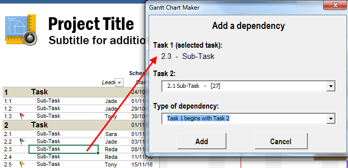
METHOD 2: SET A DEPENDENCY BETWEEN TWO NON-ADJACENT TASKS

If the two tasks are not adjacent, it is still possible to create a dependency:

Select the row of the subject task
Right click or ribbon menu -> « Dependencies »
Choose « Customized dependency »
« Task 1 » correspond to the task selected from the previous step
Choose the « Task 2 » from the drop down list
Select the desired dependency from the drop-down list
Click « ADD »

METHOD 3: SET A DEPENDENCIES WITH FORMULAS

For more flexibility, you can opt to set-up simple formulas to link different tasks or sub-tasks:

Select the cell that contains the « Start Date » that you would like to modify
Write the symbol equal « = »
Select any other date (« Start Date » or « End Date »)
Write +1 (to add one day)
Confirm by pushing « Entry » key

Based on the above example; you can play with this formula by adding or substracting more or less than 1 day. Also, instead of linking to the previous sub-task, you can make a link with any other cell of your table.

For example, if you would like to start a sub-task after the previous one, these are the steps to follow: Did you find a solution to your question ? Link to the contact form Back to the top of the page

Question 35

Is it safe to pay on this website ?

ammaranass · Accepted Answer

In order to offer the safest purchase experience we use Sellfy and Paypal. These two platforms are the leaders of digital e-commerce. The financial transaction is exclusively handled by Paypal, an industry leader that has been in existence for more than 10 years and helps protect your credit card information with the best systems and fraud prevention. At no time we have access to your payment information or those of your credit card. Everything is handled by PayPal and once your payment is processed Sellfy is notified and will send you a link to download your purchase. Did you find a solution to your question ? Link to the contact form Back to the top of the page

Question 36

Do I need a PayPal account ? Which payment methods are accepted ?

ammaranass · Accepted Answer

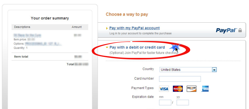
If you have a Paypal account, you can use it and speed-up the check-out process. However, a Paypal account is not required for the payment if you don't have one. When you reach the check-out page, choose the option "Pay with a debit or credit card" :

Did you find a solution to your question ? Link to the contact form Back to the top of the page

Question 37

Contact Form

ammaranass · Accepted Answer

If you did not find an answer to your question from the above information, feel free to contact us using the following form:

[contact-form to='contact@mgt-tools.com' subject='(Support) Support Gantt Chart Maker'][contact-field label='Name' type='name' required='1'/][contact-field label='Email' type='email' required='1'/][contact-field label='Your question is related to' type='select' required='1' options='STARTER Version, PRO Version, BUSINESS Version, Payment & Reimbursement, Others'/][contact-field label='Which Excel version do you use ?' type='text'/][contact-field label='Which type of computer are you using ?' type='select' options='PC,MAC,Others'/][contact-field label='Which issue are you facing ?' type='textarea'/][/contact-form]

<hr />

Getting Started:

How to Add New Rows ?

How to Change the Starting date of the Gantt Chart ?

How to Input the Start Date of a Task ?

How to Input a Duration ?

How to Update the Progress Status of a Task ?

How to Assign a Responsible Person ?

How to re-number the tasks ?

How to Modify the « Baseline » Date ?

How to Force the Gantt Chart to Refresh the View ?

How to Change the Language ?

How to Show and Fill Budget Fields ?

How to Show/Hide the Column for « Comments » ?

How to Automatically Share the Latest Schedule by Email ?

How to add a new gantt chart in the same file ?

How to Reach the support page from the Gantt Chart Maker ?

Is it possible to input task durations in weeks or months ?

What is the purpose of a “Milestone”

How to copy/paste tasks between different gantt charts ?

I can’t see the ribbon menu (Excel 2007 & Mac 2008)

Customize your Gantt Chart :

How to Show the Chart Weekly, Daily, Monthly, Quarterly ?

How to Change Project Title and Logo ?

How to Add a Flag to a Tasks ?

How to Modifiy the Way Weeks Numbers are Displayed ?

How to Automatically Adjust Print Margins ?

How to Modify Working Days (week days) ?

How to Modify Holidays and Vacations ?

How to extend the Gantt Chart period ?

How to hide the left menu ?

Advanced Questions:

How to migrate to a new version of the tool ?

How to repair formulas ?

How to Activate/Deactivate the Reminder about « Enable Macros »?

How to Customize the Colors Used in the Gantt Chart?

How to customize the pre-defined colors of « one color per person in charge » ?

How to set dependencies (or constraints) between tasks ?

Order and Payment FAQ:

Is it safe to pay on this website ?

Do I need a PayPal account ? Which payment methods are accepted ?

Contact Form:

Contact Form